

When you are computing your grades in Excel, you’re capable of utilizing multiple nested IF statements in Excel. These IF statements let you determine the letter grades using a percentage score. Although, this approach can be quite complex. Fortunately, Microsoft introduced a more straightforward alternative in 2016 called the IFS function. While using the IFS function, you can proficiently combine all conditions into your single function. This approach has made your grading much easier to comprehend.
Easiest Method: GWA Calculator
However, these nested IF formulas of Excel’s grading system assess specific conditions and assign your corresponding grades. Let’s consider a scenario where we have a dataset comprising %age scores, and our objective is to determine your corresponding grades. In this case, we can simplify the complicated calculations by employing the more user-friendly approach of utilizing multiple nested IF formulas in Excel. So, this method allows us to efficiently handle all the specified conditions while arriving at the desired results.
CHECK: How to Compute Grades in Card?
You may notice these two noteworthy facts about the grading in Excel:
Contents
Computation of grades in Excel
How to Compute Grades in Excel? You can understand this grading method in Excel formula sense by going through the following examples:
Example: Compute your Grades in Excel Formula
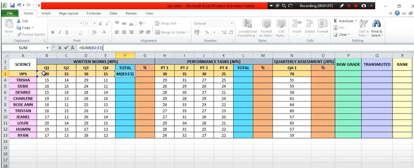
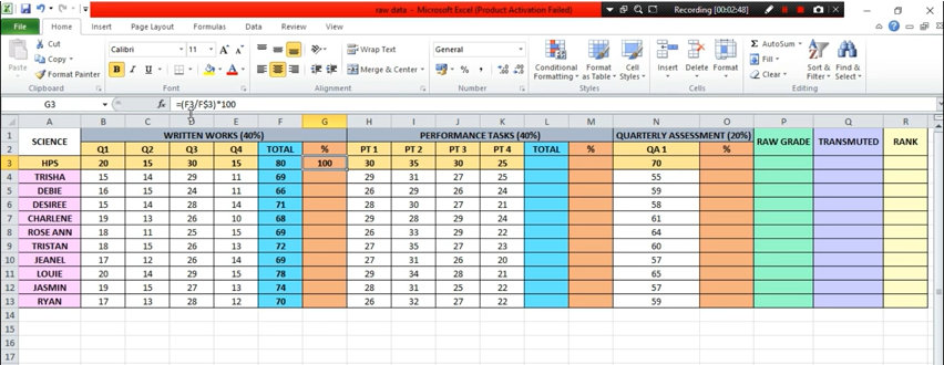
Here we have the actual data comprising the final exam marks of students for their Excel grading. Our objective is to compute the corresponding grades according to these marks. Hence, we have established specific criteria for assigning grades and have successfully calculated the grades. Your remarkable feature is to remember the highest marks correspond to an “A” grade, while the lowest marks with a “D” grade.
Here you have the following instructive steps for applying this method:
= IF (H2>80%,”A”,IF(H2>70%,”B”,IF(H2>60%,”C””D”)))
Hence, this formula represents that “if your %age is higher than 80. You are leading in the Grade A range.”
CHECK: DepEd Grading System Philippines
= IF (H2>80%,”A”,IF(H2>70%,”B”,IF(H2>60%,”C””D”)))
Meanwhile, if your %age is coming in the range of 70, then you’re falling in the Grade B range.
==IF (H2>80%,”A”,IF(H2>70%,”B”,IF(H2>60%,”C””D”)))
%age is higher than 60, and the student comes in the grade C range.
== IF (H2>80%,”A”,IF(H2>70%,”B”,IF(H2>60%,”C””D”)))
Students with %age lower than 60 will occupy Grade D (lowermost).
== IF (H2>80%,”A”,IF(H2>70%,”B”,IF(H2>60%,”C””D”)))
Example: Compute your Product Quality Grades in Excel Formula
You are capable of determining the fruit quality grade based on their quality scores according to the Excel formula. The highest quality score comes to an excellent grade of A, while the lowest quality score is D.
> = IF (B2>80%,”A”,IF(B2>70%,”B”,IF(B2>60%,”C”,”D”)))
The logical definition is here “Suppose %age is higher than 80, and your product comes in the Grade A category” as:
= IF (B2>80%,”A”, IF(B2>70%,”B”, IF(B2>60%,”C”,”D”)))
Hence, with 70 percentage, your product falls into the Grade B category for 70%:
=IF(B2>80%,”A”, IF(B2>70%,”B”, IF(B2>60%,”C”,”D”)))
With %age higher than 60, Grade C is allotted to this product:
=IF(B2>80%,”A”,IF(B2>70%,”B”,IF(B2>60%,”C”,”D”)))
Lastly, with % an age lower than 60, Grade D is allotted to a related product:
=IF(B2>80%,”A”,IF(B2>70%,”B”,IF(B2>60%,”C”,”D”)))
“=IF(AND(B2>=90,C2>=90,D2>=90,E2>=90),“Excellent”,“Satisfactory”)”
“=IFS(B2>550,”A”,B2>500,”B+”,B2>400,”B”,B2>300,”C”,B2<300,“FAIL”)”
“=IF(B2>550,”A”,IF(B2>500,”B+”,IF(B2>400,”B”,IF(B2>300,”C”,“FAIL”))))”
“= IF (A2>=35, “PASS”, “FAIL”)”
Notable Facts of Excel Grading Computation
Ultimately, you need to press your required cell, that’s compatible with your data. You can insert your letter grade. Next, you may tap on the Insert Function icon that opens a dialogue box forefront to you. ‘Search for your function’, write “IFs”, and press ‘Go’.
Now from ‘Select Function’, open your IFs by double-clicking on it. Insert the cutoffs for each letter grade, starting with the bottom cutoff for grade A. Proceed with entering the cutoffs for subsequent grades and acquire your required percentage grade.